Implementation

Note: the formulae in this section are in laTEX format, which is slightly different from the native reStructuredText format. Therefore, some formulae may display incorrectly. You can check the source and copy the formula if needed.

The system was implemented as a micro-service Python package. It provides its functionality through several public-facing methods, the Application Programming Interface (API).

Calling one of the API methods gives back a JSON-like response (a dictionary in Python) with additional information appended to what was received. The additional information can be:

• A normalised value in each parameter of a bike geometry without additional symbols or letters and in a standard common format and metrics (degrees or millimetres).
• Additional parameters of a bike geometry that were missing and that could be derived from others.
• Calculated values for all the parameters of the bike geometry that could be validated.
• A confidence score for each parameter as a percentage from 0 to 1 depicting how likely this parameter fits with the rest of the bike geometry.
• A confidence score for each bike geometry as a percentage from 0 to 1 depicting how likely all the bike parameters fit together and the likelihood of the bike being mathematically plausible.

The confidence scores range from 0 to 1 inclusive, where:

• 0, the lowest value, means that the parameter and/or bike geometry do not fit together at all and it is very likely that there is something wrong;
• and 1, the highest value, means that the parameter and/or bike geometry fit perfectly and are very likely to be mathematically correct.

This section focuses on the technical details of the package developed, its components, the automated test framework and the deployment of it in production environments.

System Overview

The system was built as a Python 3 package and it can be deployed as a micro-service in serverless computing environments. A serverless computing environment allows to run services in production without worrying about servers, maintenance or scaling, and only paying for the computing time used. The provider handles all of this for you and the code is only executed when it receives a request to do so (e.g. a HTTP request). It is common way of running event-driven code on-demand that scales as you need it to, whilst reducing the cost of running a server 24 hours a day. Examples of serverless environments are Google Cloud Functions and Amazon Web Services Lambda (AWS Lambda).

As mentioned above, we have provided a public API to access the functionality. Given a JSON representation of a bike geometry (or multiple geometries), it normalises the parameter values, validates the geometry and returns the same representation with additional fields added.

The system does not have a front-end or graphical user interface to interact with it. It is a back-end only system which can be plugged into other systems as required.

Furthermore, as the system is a Python 3 package, we named it “datavalidation” following Python’s recommended style for package names. The rest of this section may also refer to the system as the datavalidation package.

Architecture

The system can be divided into four well-defined parts:

1. The public API, which contains the public methods and the logic to glue the other modules together.
2. The core module, which contains package-wide functionality and defines objects to hold bike geometries and its parameters.
3. The normalisation module, which contains the logic to normalise parameter values.
4. The validation module, which contains the logic to calculate geometry parameters and validate bike geometries.

The normalisation and validation modules depend on the core module, but not vice-versa. These modules are also independent from each other to allow greater flexibility when one of them needs to be modified. Figure 1 below shows the system architecture of the datavalidation package and the dependencies between the modules. It also includes the only external dependency of the package, the SymPy library.

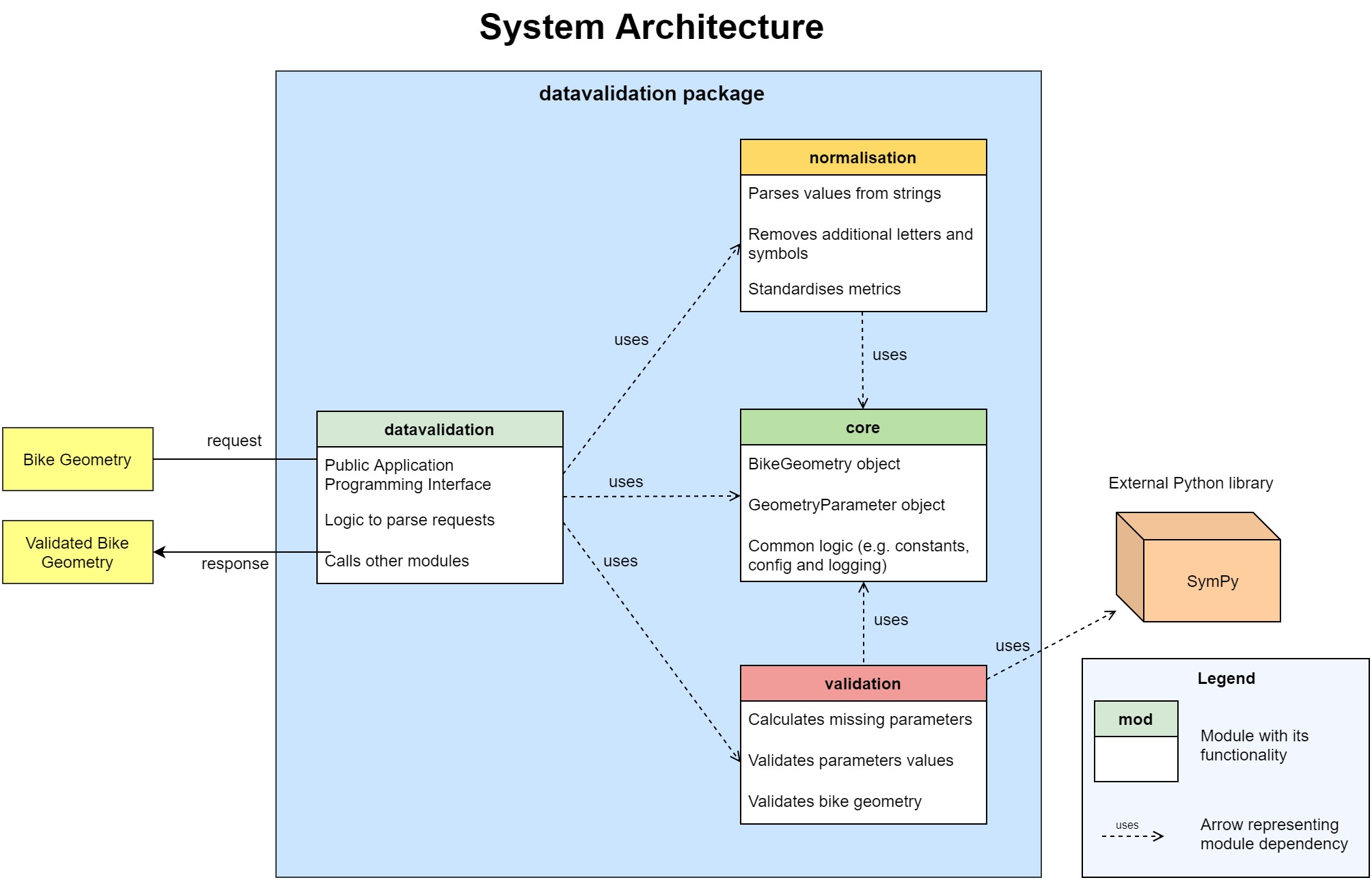
Figure 1: System architecture of the datavalidation package

An additional file, a Flask wrapper, is delivered with the rest of the system, but it is not part of the datavalidation package and it is only used to show how easy it is to deploy in an AWS environment. Section Deployment gives more details of this file.

Information Flow

Figure 2 shows a flow chart of the main function of the system: validate bike geometries. It shows how the process is executed as a pipeline and where each module fits within the whole system.

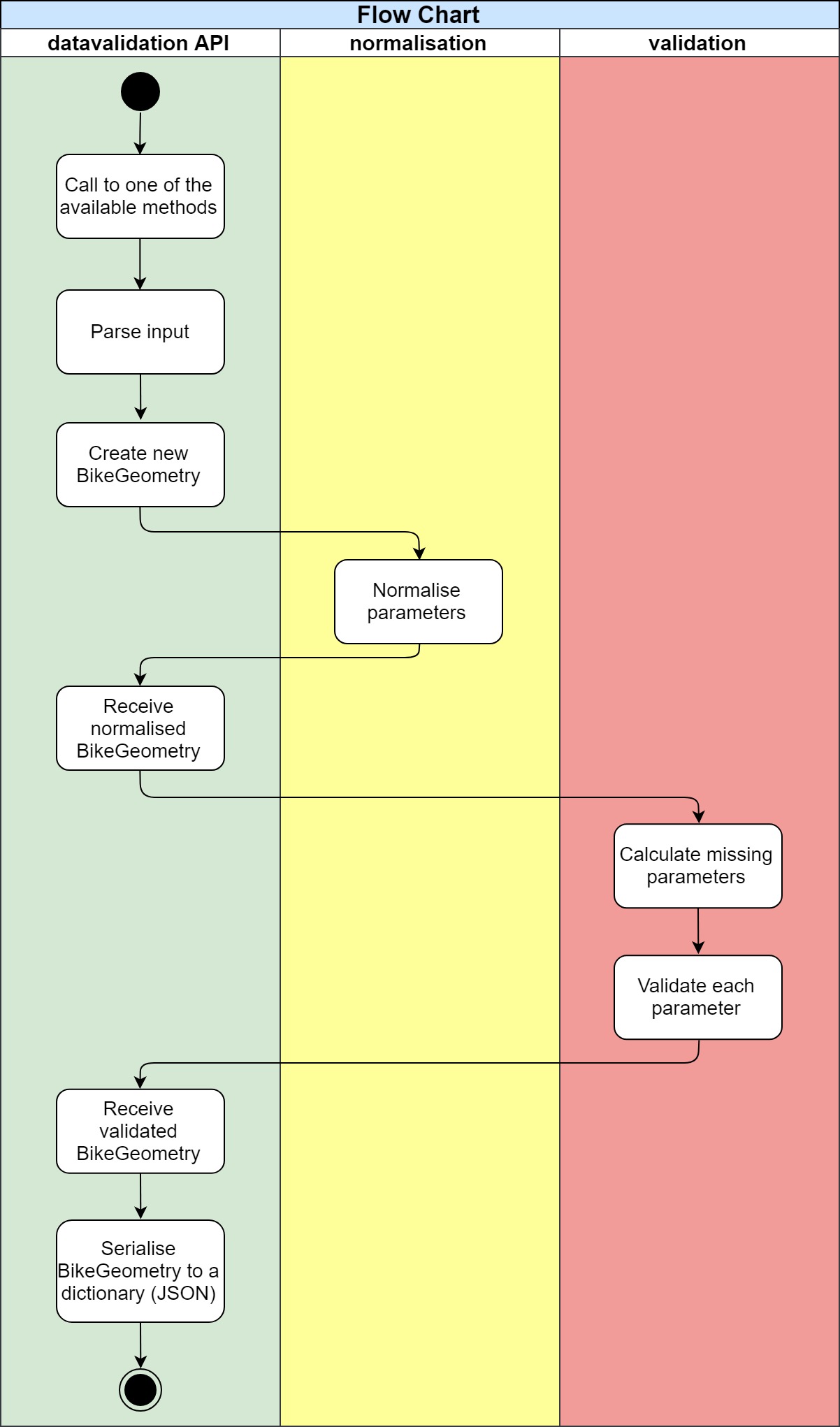
Figure 2: Flow chart for the datavalidation package

The process starts when one of the public API methods is called with a bike geometry. This bike geometry is in a dictionary, a structure very similar to JSON in Python. The main datavalidation module parses it and creates a new BikeGeometry object that holds information about the bike and its parameters. This BikeGeometry object is declared in the core module of the package, so the other modules have access to it too.

The datavalidation module passes the BikeGeometry to the normalisation module, which normalises the values of the parameters and puts them in an standard format. Then, the normalised BikeGeometry is returned to the main module, and this one passes it to the validation module.

The validation module uses several submodules to calculate missing parameters and validate the BikeGeometry. First, it calculates the missing parameters by deriving them from others (e.g. derive “chainstay” from “wheelbase” and “bb_drop”). This process loops until no more parameters have been calculated in the previous iteration (sometimes deriving one parameter opens the possibility to derive more). Then, each parameter is validated individually by calculating it using several equations and averaging the deviation from the results. If some parameters cannot be calculated, it uses the geometry constraints and statistics to derive a rough deviation from their median and mean. Next, the BikeGeometry calculates its confidence score using its parameter’s confidence. Finally, the datavalidation module serialises the BikeGeometry into a dictionary and returns it as the final result.

Modules

This section goes through the various modules and components of the system from Figure 1. All the modules are in Python 3.

The datavalidation Module

This is the main module of the system that provides the public methods of the API. Calling one of these methods will make the system validate the given bike geometry and return the results of said validation.

Its primary function is to control and glue the other modules together to provide the high-level functionality of the package. It uses the core module to parse and create the BikeGeometry objects that will be used by the normalisation and validation modules. It calls methods from these last modules as needed.

It is also responsible for assembling the final response based on the results of the validation on the BikeGeometry object.

The core Module

This module provides definitions for commonly used methods and objects, most notably the BikeGeometry and its GeometryParameters. It also has the logic for setting up the package configuration, the logging and several constants. The most important objects declared in this module are defined below:

• BikeGeometry: object that holds information about a bike geometry, including its parameters and certain config options. It also provides logic to work with bike geometries and to convert from/to JSON representation.
• GeometryParameter: object that holds information about a parameter of a BikeGeometry. It contains several utility functions to retrieve the parameter value, its type, confidence, calculated value, etc.

The normalisation Module

This module normalises the values of the parameters inside the bike geometry. It has an internal architecture similar to a pipeline: it first checks for multiple values (e.g., “70 / 80”); then for numbers (e.g., “70mm”) and finally, it performs some basic measure checks to put everything in millimetres if possible.

The aim is to obtain a common representation of the value that can be used safely across the rest of the package without worrying about types or additional characters. The BikeGeometry and GeometryParameter objects encapsulate this common representation as it may change over time when new information is added (e.g., normalised value, calculated value and original value).

The validation Module

This module controls the validation process. It uses several submodules to validate BikeGeometries and GeometryParameters, and calculates the GeometryParameters missing if possible. The execution order is given in the Information Flow Section.

The results of validating a BikeGeometry are:

• The GeometryParameters from inside the BikeGeometry that could be validated now have confidence values.
• Some GeometryParameters may be deemed invalid due to low confidence values.
• Some GeometryParameters may have new calculated values, even if the previous values were valid.
• Some GeometryParameters without a value may have a new value calculated by deriving it from others.
• The confidence value of the BikeGeometry can now be calculated.

Refer to Section Mathematical Model for more information on the equations used to calculate values.

Confidence Values

The confidence score represents how likely a parameter or bike geometry makes sense and it is mathematically plausible. The confidence score range from 0 to 1 inclusive, where:

• 0, the lowest value, means that the parameter and/or bike geometry do not fit together at all and it is very likely that there is something wrong;
• and 1, the highest value, means that the parameter and/or bike geometry fit perfectly and are very likely to be mathematically correct.

A bike geometry is said to be invalid if its confidence score is below some threshold, set by default to 0.7 but configurable through the API input. Similarly, the parameters of the bike geometry may be invalid if they are below this threshold too. This is all included in the response of the datavalidation package.

Validating Parameters

There are two distinct validation methods for:

1. Calculating the value of the parameter using equations from the mathematical model and then comparing it to the current value. The division between these two values gives an absolute percentage of how far away the current value is, which becomes the confidence value of the parameter. Because the difference is relative to the values of the parameters themselves, the larger the values are, the more tolerant that they are to variations (e.g., a deviation of 1% in 1000 mm is 10 mm, whereas the same deviation in 100 mm is only 1 mm). The formula is:

\[\begin{split}Confidence(x) = \\ x_{current} / x_{calculated} & \quad \text{if } x_{current} <= x_{calculated} \\ (x_{current} / x_{calculated}) - 1 & \quad \text{if } x_{current} > x_{calculated}\end{split}\]

In some cases, the result may be outside the range [0-1], so it is rounded to the nearest edge (e.g., when one of the values is twice or three times the other due to some error).

2. Some bike geometries may not have enough parameters to validate other parameters such as described above. Instead, we use geometry statistics that we extracted from many bike geometries. The data was dirty (values missing, bikes with hundreds of meters long, etc.), thus the automated process that we used yielded extreme values for some parameters. Therefore, when using the geometry statistics, we average the deviation of the parameter from both its mean and median. Although this is a simple and crude process, it showed promising results in calculating acceptable confidence scores for some parameters. The formula is:

\[Confidence(x) = \frac{deviation(x, mean(x)) + deviation(x, median(x))} {2}\]

Validating Bike Geometries

To validate bike geometries, we calculate its confidence score based on the combination of the confidence score of its parameters. We implemented three different algorithms to calculate this score with each having a different level of strictness over the geometry. These are:

1. Optimist: computes the arithmetic mean of the parameters’ confidence. As it only counts those parameters that were validated, it often gives high confidence values when in fact most of the bike geometry is just missing. The formula is:

\[BikeConfidence(x) = \frac{1}{n} {\displaystyle\sum_{i=1}^{p} confidence(p_i)}\]

where p is a validated geometry parameter

2. Pessimist: computes the sum of all parameters’ confidence divided by the total number of parameters that we can validate using the equations. This number is 13 at the moment. Calculated missing parameters are not counted in the sum, so it often gives low confidence values even when the bike geometry is correct mathematically overall. The formula is:

\[BikeConfidence(x) = \frac{\displaystyle\sum_{i=1}^{p} confidence(p_i)} {\displaystyle\sum_{i=1}^{p} {validatable\_} p_i}\]

where p is a validated geometry parameter

3. Realist: computes the sum of all parameters’ confidence divided by the total number of parameters that we can validate using equations. This algorithm counts calculated missing or invalid parameters in the sum to produce slightly higher results than the pessimist variation. The confidence value for invalid or missing parameters is capped at 0.65 (usually much lower), thus it does not produce unrealistic confidence score such as with the optimist algorithm. It calculates confidence values in the range between the optimist (best case) and pessimist (worst case) algorithms above. We found that this algorithm is on the sweet spot for many bike geometries, since it does not punish geometries that have missing values which can be derived. The formula is:

\[BikeConfidence(x) = \frac{ \sum_{i=1}^{p} confidence(p_i) }{ \sum_{i=1}^{p} {validatable\_} p_i }\]

where p is a validated, derived or calculated geometry parameter

We found that the third algorithm computes the best or most realistic results, thus it is used by default to calculate the confidence score of a bike geometry. You can provide a flag in the input geometry of the datavalidation package to select a different algorithm. This is detailed in the technical guide.

Mathematical Model

We were able to link the most important bike geometry parameters through several equations. The collection of these equations and how they relate to bike geometries is what we call the mathematical model of a bike geometry. During the validation process, the system uses these equations to calculate values for parameters through others. The comparison of the current and calculated values also helps computing confidence scores.

There are a total of six equations implemented, each linking from three to six parameters at the same time. All the equations are equalled to zero as this makes it easier to reorganise them as needed. The equations assume that the parameters values are in millimetres (if a length) and degrees (if an angle).

The equations were derived using a combination of geometry formulae including trigonometry. They were then thoroughly tested with distinct types of bike geometries and accepted if the error was minimal in every type of geometry, or discarded if they did not perform well in some geometries. The equations are:

Equation 1:

\[(top\_tube - stack) \cdot tan(radians(90 - seat\_angle)) - reach = 0\]

Equation 2:

\[\sqrt{(bb\_drop)^2 + (wheelbase - \sqrt{(front\_centre)^2-(bb\_drop)^2})^2} - chainstay = 0\]

Equation 3:

\[\sqrt{(seat\_tube\_length\_effective)^2 - (stack)^2} + reach - top\_tube = 0\]

Equation 4:

\[\begin{split}bb\_drop - stack + sin(radians(head\_angle)) \cdot \\ (head\_tube + fork\_length - fork\_rake \cdot cos(radians(head\_angle))) = 0\end{split}\]

Equation 5:

\[(\frac{stack}{cos(radians(90 - seat\_angle))}) - seat\_tube\_length\_effective = 0\]

Equation 6 (split across multiple lines):

\[radians(atan2(\frac{ stack - bb\_drop }{ \sqrt{(front\_centre)^2-(bb\_drop)^2 }) - reach - fork\_rake)}) - head\_angle = 0\]

The parameters that we are able to calculate from these equations are the following 13:

• bb_drop
• chainstay
• fork_length
• fork_rake
• front_centre
• head_angle
• head_tube
• reach
• stack
• seat_angle
• seat_tube_length_eff
• top_tube
• wheelbase

We investigated other equations, but they were not as robust as the equations listed above with distinct types of bike geometries (e.g., mountain bikes, road bikes, etc.). The error of the implemented equations is often minimal when compared to the actual values of the geometries, often a few millimetres or less than two degrees off. We think that this error is due to a combination of floating point precision and the bike geometries being rounded to nice values (the values are often natural numbers with no decimals, and usually in “pleasing” numbers, e.g., 425mm, 70 degrees, etc.). Future work should look into deriving additional equations to improve the robustness of the mathematical model.

Furthermore, some equations would have more than one solution when calculating one parameter (e.g., square root has both a positive and a negative result). We introduced the geometry constraints to filter the solutions of an equation to a manageable number.

Geometry Constraints

The geometry constraints are triples that enable the system to perform “common sense” checks on geometry values. Parameters of a bike geometry may constraints that relate it (or constraint it) to another parameter.

Each triple has the form “subject predicate object”, where both the subject and object refer to geometry parameters, whilst the predicate details the relationship between them. An example geometry constraint is chainstay < wheelbase, which constraints the chainstay of a bike geometry to always be smaller than the wheelbase.

The geometry constraints are always complemented by their opposite in the object parameter. This enables the system to filter away solutions to equations that do not satisfy these constraints. For instance, geometry constraints are essential to filter solutions in equation number 2, where chainstay often has multiple solutions due to the square roots, e.g., chainstay = [-200, 200, 500, 1500] becomes chainstay = [500] when filtering negatives and applying the constraints (these are not real values).

Finally, the geometry constraints also have safety checks through the geometry statistics mentioned in the Validation Module Section. The constraints can be ambiguous regarding which value makes the constraint fail (e.g., chainstay may be fine, but wheelbase is 100mm instead of 1000mm due to a typo). If a geometry constraint evaluates to false, it also checks which value is more likely to be wrong (either chainstay or wheelbase) by looking at the geometry statistics of that value. Only the value which is likely to be wrong is flagged as such in a pair of geometry constraints.

Testing

Testing is an integral part of the system. It was developed with Test Driven Development (TDD) to make sure that additional features did not compromise the robustness and integrity of the system. In TDD, the programmer codes the tests before writing the actual code that satisfies them. Therefore, it requires finding the final goal of a feature before it is implemented. For instance, we wrote what we wanted to achieve from the normalisation module before working on it, coding tests that checked that the result of normalising “190,5mm” was “190.5”.

The requirements of the system drove the development of the acceptance tests. These are the tests that check a whole requirement (e.g., a test to check that normalisation in a bike geometry gives expected results). However, most of the tests were unit tests that checked the logic of single functions. There were also a few integration tests that tested the whole system.

The tests were automated using PyTest, a package that offers a framework for testing projects in Python 3. Each file in the datavalidation package has its own test file that performs checks on it, ensuring the results are always correct even on the edge cases.

Deployment

There are different ways of deploying the system into a production environment that GeometryGeeks can use. The most obvious one is in a serverless environment, such as Amazon Web Services (AWS) Lambda or Google Cloud Functions. Since these type of environments are ideal for the system developed as a Python package.

To asses the system outside our development and testing domain, we deployed in into an AWS virtual machine (a server in other words). The entire process took less than 10 minutes to complete and we used this system during the demonstration.

The deployment process to the AWS virtual machine consisted in 3 steps:

• Installation of Python version 3.6.
• Installation of system requirements from the texttt{data-validation/requirements/prod.txt} file and only the Flask requirement from texttt{data-validation/requirements/dev.txt}.
• Starting the server by running the command texttt{python3 flaskwrapper.py}.

Overall, the entire deployment of the system requires two modules to be installed. This allows the user to transfer the system easily in a small amount of time.